TL;DR.
A paper posted on October 1 asked a question that every model router, cascade and speculative decoder depends on, and that nobody had measured: how much compute does each token actually need?
The answer, from researchers at Duke and the University of Washington, is lopsided. On math and code benchmarks, a 0.5B model reproduces 92 to 95% of the tokens in a verified answer written by a 72B model. The remaining few are expensive: the costliest 10% of tokens account for 64 to 80% of the estimated compute.
That sounds like a 90% discount waiting to be collected. It isn't, and the paper's own appendix shows why:
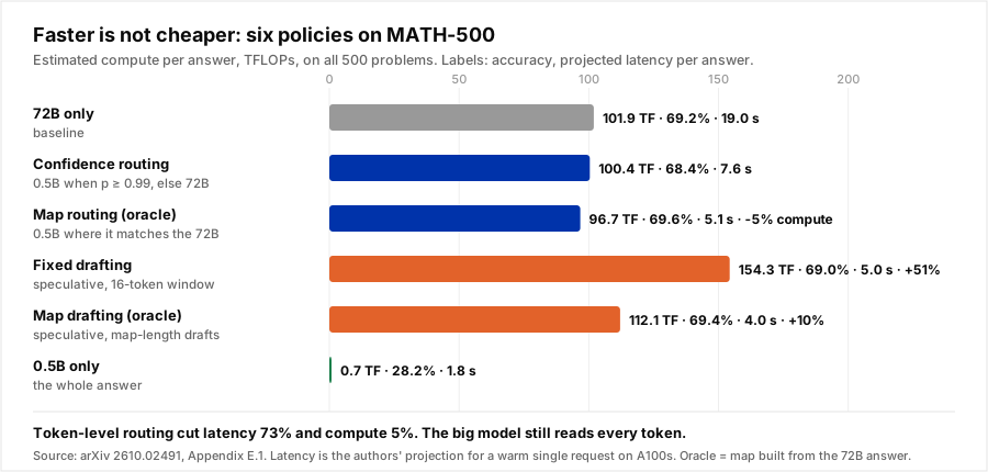
- Routing token by token cut latency 73% but compute only 5%. On MATH-500, sending each token to the 0.5B model wherever it would match the 72B brought projected time per answer from 19.0 to 5.1 seconds. Compute went from 101.9 to 96.7 TFLOPs, because the big model still has to read every token the small one writes.
- Speculative decoding was faster and used more compute, 10 to 51% more than running the 72B alone.
- The 0.5B model alone used under 1% of the compute and scored 28.2% instead of 69.2%. 95% easy tokens did not make 95% easy answers.
This post walks through what the paper measured, why the savings live at the level of whole requests rather than tokens, and a Python tutorial that runs the same test on your own traffic: token agreement against task success, and what each one would save.
Figures are from the paper as published (arXiv 2610.02491, v1). The cost example in the last section is illustrative and priced at October 7, 2026 list prices. None of this is Nadir customer data.
What the paper measured.
What Does a Token Cost? by Zhixu Du, Weijia Han, Hai Helen Li and Yiran Chen builds a panel of fifteen open models in three families: Qwen2.5 from 0.5B to 72B, OLMo-2 from 1B to 32B, and DeepSeek-R1-Distill-Qwen from 1.5B to 32B. A large model writes an answer, a checker confirms it's correct, and then every model in the panel is shown the correct text one token at a time and asked to predict the next token.
For each position, the sufficient compute is the cost of the smallest model that predicts the right token. It's an upper bound on what that token needed. A small model reproducing a token is the condition every efficiency trick assumes: a router hopes a small model can write the whole answer, a speculative decoder hopes it can draft the next few tokens, and a token-level cascade hopes it can write this one.
The setup covers GSM8K, MATH-500 and HumanEval as the core benchmarks, with nine more for robustness, 50,019 prompts in all. References come from Qwen2.5-72B, with a second set from Llama-3.3-70B to check that the results don't depend on who wrote the text.
Most tokens are easy. Most compute is not.
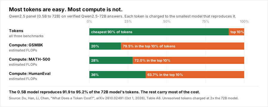
Within the Qwen2.5 panel, the 0.5B model reproduces 91.9 to 95.2% of reference tokens across the three core benchmarks. The 1B OLMo and 1.5B R1-distilled models land at 89 to 92%. It holds across families.
The cost sits in the tail. Ranked by sufficient compute, the most expensive 10% of tokens account for:
| Panel | Top 10% of tokens, share of compute | Top 1% of tokens |
|---|---|---|
| Qwen2.5 | 63.7 to 79.5% | 52.9 to 60.1% |
| OLMo-2 | 63.8 to 69.4% | 16.3 to 19.9% |
| R1-Distill-Qwen | 67.2 to 74.8% | 11.5 to 15.0% |
In the Qwen panel, one token in a hundred carries more than half the compute. Those are the positions where only the 72B model, or no model in the panel, gets it right.
Two more findings matter for anyone building a router:
Families agree on which tokens are hard. After controlling for surprisal and position, Qwen, OLMo and Falcon rank positions by difficulty with partial correlations of 0.32 to 0.48. Hard tokens are partly a property of the text, not only of the model reading it. The authors are careful to say this doesn't yet show that a difficulty map built with one family transfers to another.
You can't spot hard tokens by looking at them. Word length, digits, operators, frequency and position together explain only 2.5 to 3.2% of the variation in which tokens need a bigger model. The difficulty is in the context. Simple surface rules are weak at the request level too, which is why we spend so much time on calibration.
Why 95% easy didn't become 95% cheaper.
The authors then gave two controllers an oracle: the map of exactly where the 0.5B model matches the 72B on every one of the 500 MATH-500 problems. No real system has that map in advance, so these are upper bounds on what token-level allocation can do with these two models.
| Policy | Accuracy | Projected time per answer | Compute (TFLOPs) | Compute vs 72B only |
|---|---|---|---|---|
| 72B only | 69.2% | 19.03 s | 101.92 | baseline |
| Confidence routing, θ = 0.99 | 68.4% | 7.59 s | 100.38 | -1.5% |
| Map routing (oracle) | 69.6% | 5.12 s | 96.71 | -5.1% |
| Fixed drafting, 16 tokens | 69.0% | 4.98 s | 154.30 | +51.4% |
| Map drafting (oracle) | 69.4% | 3.99 s | 112.07 | +10.0% |
| 0.5B only | 28.2% | 1.84 s | 0.67 | -99.3% |
Read across the compute column and the headline flips. The oracle router matched the 72B's accuracy, beat the best confidence-threshold cascade by 1.2 points and 2.5 seconds, and saved 5% of the compute.
The reason is in how the authors count. Every time the 72B takes over after the 0.5B has written a stretch, it has to process those tokens into its own cache before it can predict the next one. Reading a token costs a model about as many FLOPs as writing it. What's different is time: the 72B reads a block of tokens in one parallel pass, while it writes them one at a time. So handing easy tokens to a small model saves mostly waiting, not arithmetic. Speculative decoding makes the same trade more aggressively: the big model verifies drafts it would otherwise have generated, and rejected drafts are pure extra work. We made the same point from the billing side in speculative decoding: faster isn't cheaper.
Whether that time saving is a cost saving depends on what you pay for. If you rent a GPU per hour and serve one request at a time, latency is your bill and a 73% cut is real. Under heavy batching, the GPU stays busy either way and FLOPs move closer to cost. The paper's latency figures are a projection for a warm, single-request setup on A100s and don't model batched serving, so read them as a ceiling for that case.
If you buy tokens from an API, token-level routing isn't on the menu at all. You can't swap providers in the middle of a decode, and every handoff between models sends the full prefix again as input, usually without a cache hit. That's the switch penalty.
Cheap tokens, expensive mistakes.
The second experiment explains why you can't simply let the small model run on the easy stretches.
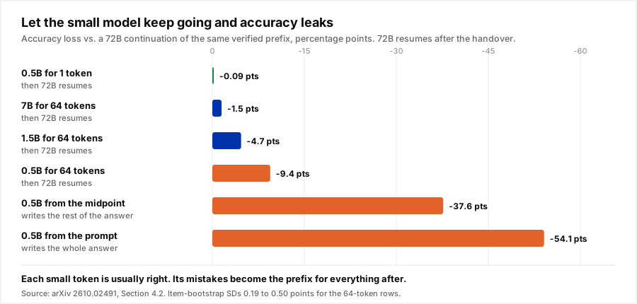
The authors let a small model write for a fixed number of tokens on its own, then handed the text back to the 72B. One token from the 0.5B model costs nothing measurable, -0.09 points. Sixty-four tokens cost 9.4 points. A 7B model writing the same 64 tokens costs 1.5. Letting the 0.5B write the whole rest of the answer from the halfway point costs 37.6 points, and from the start, 54.1.
The token-reproduction number is measured with the correct text in front of the model every time. In free generation, the small model's rare mistakes become the prefix for everything after, and they compound. This is the core reason a cascade needs a check on the finished answer, not a guess at the start, and why shepherding a small model with a few big-model tokens works better than handing off halfway.
What this means if you're paying the bill.
Put the two experiments together and the picture for anyone buying inference is clear.
The savings are at the request level. Look at the last row of the table. Running the 0.5B model for the whole answer used 0.66% of the compute and got 28.2% of problems right. For a router that could pick out those 141 problems in advance, that's the entire cost of the 72B avoided on each of them, not 5% of it. The per-token map says small models are good at almost every step. The per-request result says they finish some tasks completely and fail others badly. A request router doesn't need to know which tokens are hard. It needs to know which requests a cheaper model will finish correctly, and send only those down. That's the decision FrugalGPT and RouteLLM were built around, and the one this paper's own related-work section places at the coarse end of the same spectrum.
Agreement is not success. A cheap model that writes text that looks like the frontier model's 95% of the time is not a model that solves 95% of your tasks. If you evaluate a downgrade by comparing outputs with something like token overlap or BLEU against the expensive model, you'll overestimate how much traffic can move. Measure task success with a checker.
Long handoffs cost quality. Any design where a cheaper model writes a long stretch and a stronger model "cleans up" pays for the compounding error the handover experiment shows. If you escalate, escalate the whole request, and account for the retry tax.
Finer-grained routing is real, but it lives inside serving stacks. If you self-host both models on the same GPUs, token-level policies are worth testing for latency. Above the API, the finest grain worth routing at is usually the subtask or agent step, not the token.
Tutorial: token agreement vs task success on your own traffic.
This runs the paper's measurement on a sample of your production requests, then checks the claim that matters for the bill. You need prompts with a reference answer from the model you use today, a way to check correctness (unit tests, an exact-match answer, or a rubric), and a small open model. A laptop CPU handles a 0.5B model on a few hundred prompts. A GPU is faster.
Step 1: build the agreement map.
Feed the small model the prompt plus the reference answer and record, at each position, whether its top prediction matches the reference token. This is teacher forcing: one forward pass per request, not one per token.
import json, statistics
import torch
from transformers import AutoTokenizer, AutoModelForCausalLM

SMALL = "Qwen/Qwen2.5-0.5B-Instruct"
tok = AutoTokenizer.from_pretrained(SMALL)
model = AutoModelForCausalLM.from_pretrained(SMALL, dtype=torch.bfloat16)
model.eval()

def prompt_ids(prompt):
    text = tok.apply_chat_template([{"role": "user", "content": prompt}],
                                   tokenize=False, add_generation_prompt=True)
    return tok(text, return_tensors="pt", add_special_tokens=False).input_ids

def agreement_map(prompt, reference):
    """1 where the small model's greedy next token equals the reference token."""
    p = prompt_ids(prompt)
    r = tok(reference, return_tensors="pt", add_special_tokens=False).input_ids
    ids = torch.cat([p, r], dim=1)
    with torch.no_grad():
        logits = model(ids).logits[0]
    start = p.shape[1]
    preds = logits[start - 1:-1].argmax(-1)   # prediction for each reference position
    return (preds == r[0]).int().tolist()

def longest_run(m):
    best = cur = 0
    for x in m:
        cur = cur + 1 if x else 0
        best = max(best, cur)
    return best
The reference was written by a different model with a different tokenizer, so we re-tokenize it with the small model's tokenizer. The paper aligns families at the word level for the same reason.
Step 2: let the small model answer on its own.
def small_answer(prompt, max_new_tokens=512):
    p = prompt_ids(prompt)
    with torch.no_grad():
        out = model.generate(p, max_new_tokens=max_new_tokens, do_sample=False)
    return tok.decode(out[0, p.shape[1]:], skip_special_tokens=True)

def run(sample):
    """sample: list of {"id", "prompt", "reference", "check": callable(answer) -> bool}"""
    rows = []
    for s in sample:
        m = agreement_map(s["prompt"], s["reference"])
        rows.append({
            "id": s["id"],
            "agreement": sum(m) / max(len(m), 1),
            "longest_run": longest_run(m),
            "misses": len(m) - sum(m),
            "solved": bool(s["check"](small_answer(s["prompt"]))),
        })
    return rows
Step 3: compare the two numbers.
def report(rows):
    mean_agree = statistics.fmean(r["agreement"] for r in rows)
    solved = statistics.fmean(r["solved"] for r in rows)
    print(f"mean token agreement  {mean_agree:.1%}")
    print(f"small model solves    {solved:.1%} of requests")

    # The trap: requests that look almost identical token by token, but fail.
    trap = [r for r in rows if r["agreement"] >= 0.9 and not r["solved"]]
    print(f"agreement >= 90% but failed: {len(trap)} of {len(rows)}")

    # Does agreement predict success at all? Compare the two groups.
    ok = [r["agreement"] for r in rows if r["solved"]]
    bad = [r["agreement"] for r in rows if not r["solved"]]
    if ok and bad:
        print(f"agreement when solved {statistics.fmean(ok):.1%}, "
              f"when failed {statistics.fmean(bad):.1%}")
    return solved

routable = report(run(sample))
On math and code, expect the paper's pattern: token agreement in the 90s, a much lower solve rate, and a cluster of high-agreement failures. Those are the requests where one wrong token, a sign, a variable name, an off-by-one, sinks the answer. The solve rate is the number to plan with. The agreement rate tells you how close the small model is, not how often it's good enough.
Step 4: price the request-level decision.
The solve rate tells you the most traffic a perfect request router could move. Here's what that's worth, with a fallback that re-runs failures on the bigger model:
# USD per million tokens (input, output), October 7, 2026 list prices.
PRICES = {"gpt-6.1-sol": (2.00, 10.00), "gpt-6-luna": (0.10, 0.50)}

def per_request(model, tin=2000, tout=500):
    pin, pout = PRICES[model]
    return (tin * pin + tout * pout) / 1e6

def blended(routed, miss_rate, big="gpt-6.1-sol", small="gpt-6-luna"):
    """routed: share of requests sent to the small model.
    miss_rate: share of those that fail a check and get re-run on the big model."""
    b, s = per_request(big), per_request(small)
    return (1 - routed) * b + routed * s + routed * miss_rate * b

base = per_request("gpt-6.1-sol")
for routed, miss in [(0.3, 0.05), (0.5, 0.10), (0.7, 0.20)]:
    c = blended(routed, miss)
    print(f"route {routed:.0%}, miss {miss:.0%}: {1 - c / base:.1%} cheaper per request")
At 2,000 input and 500 output tokens, a request costs $0.0090 on GPT-6.1 Sol and $0.00045 on GPT-6 Luna, a 20x gap. Routing half the requests down with a 10% miss rate prints 42.5% cheaper (illustrative, list prices). Compare that with the 5% compute the oracle token router saved on MATH-500. Coarse decisions on whole requests, made well, beat fine decisions on tokens, because a routed request skips the big model completely.
Where Nadir fits.
Nadir makes the request-level decision. Send model="auto" and a trained classifier reads each prompt and picks the tier, against the quality floor you set on the API key. It routes whole requests, so a request sent to a cheaper model never touches the expensive one, and each response reports the routing decision and its cost in the metadata. If you only want the decision, POST /v1/bucket returns simple, medium or complex with a probability for each, and you call your own providers.
The tutorial above tells you the ceiling for your traffic. Observe mode tells you what routing would actually do on it: it records the decision Nadir would have made on every request without changing a single response, so you can compare the routed share and the projected cost against your own solve-rate test before you switch anything. Start with a free key.
Conclusion.
The first direct measurement of per-token compute confirms the premise behind routing: on math and code, a 0.5B model reproduces 92 to 95% of a 72B model's tokens, and the costliest 10% of tokens carry 64 to 80% of the compute. It also shows where that premise stops paying. With a perfect map of easy tokens, token-level routing cut latency 73% and compute 5%, speculative drafting used more compute than the big model alone, and 64 tokens of unsupervised small-model output cost 9.4 accuracy points. Easy tokens don't add up to easy requests. For anyone paying per token, the savings are in sending whole requests that a cheaper model will finish correctly, measured by task success, not by how similar the text looks.
Sources: Zhixu Du, Weijia Han, Hai Helen Li and Yiran Chen, ["What Does a Token Cost? A Mixture-of-Agents Measurement of Sufficient Per-Token Compute"](https://arxiv.org/abs/2610.02491), arXiv 2610.02491, v1, October 1, 2026 (Duke University and University of Washington). Concentration figures from Section 4.1 and Table A6, with unresolved tokens charged at twice the largest model's cost. Policy comparison from Appendix E.1; latency is the authors' projection for a warm single request on A100 GPUs and excludes batching, queueing and network time. Handover results from Section 4.2. Found via [Token Cost Radar](https://jcodemunch.com/radar/2026-10-06), October 6, 2026. GPT-6.1 Sol and GPT-6 Luna list prices as of October 7, 2026, via [DEV Community's DevDay 2026 roundup](https://dev.to/axrisi/openai-devday-2026-every-announcement-with-prices-and-availability-1mbh). The routing cost example is illustrative.