TL;DR.
On October 13, GitHub took the LLM out of its generic secret detection. A remote LLM pipeline used to decide whether a string that looks like a credential in a push is a real secret. A fine-tuned ModernBERT encoder makes that call now, exported to ONNX with 8-bit quantization. GitHub reports three results against the LLM it replaced:
- More than 98% lower serving cost.
- 86% lower median scan time after a push. That made it fast enough to run before the push, in push protection.
- Better answers. Offline, precision is up 13% and recall up 19% (relative). In a customer A/B test, owner-weighted acceptance of alerts rose 11.5%.
So it's cheaper, faster and more accurate, all at once. That isn't a fluke of secret scanning. It happens whenever a generative model is doing a job whose answer is a label. Most production LLM traffic has a few of those jobs hiding in it: triage, intent detection, moderation, "is this a duplicate", "does this need a human".
This post covers why the encoder wins, how to find the classifier-shaped calls in your own logs, a working distillation recipe (labels, group split, ModernBERT fine-tune, thresholds, ONNX int8), and a break-even showing which of those calls are worth a model and which should just be routed to a cheaper LLM.
GitHub figures are from its October 13, 2026 engineering post. Cost per million calls, encoder throughput, build cost and break-even volumes are our own illustrative calculations at October 2026 list prices, not GitHub or Nadir customer data.
What GitHub shipped.
Generic secrets are the hard case. A Stripe key has a prefix and a checksum, so a regex finds it. A database password in a config file looks like any other random string. So do build IDs, checksums, test fixtures and the sample keys in docs. The engineering post by Batu Ozturkler and Shengyu Fu puts it in one line: "Context is the deciding signal."
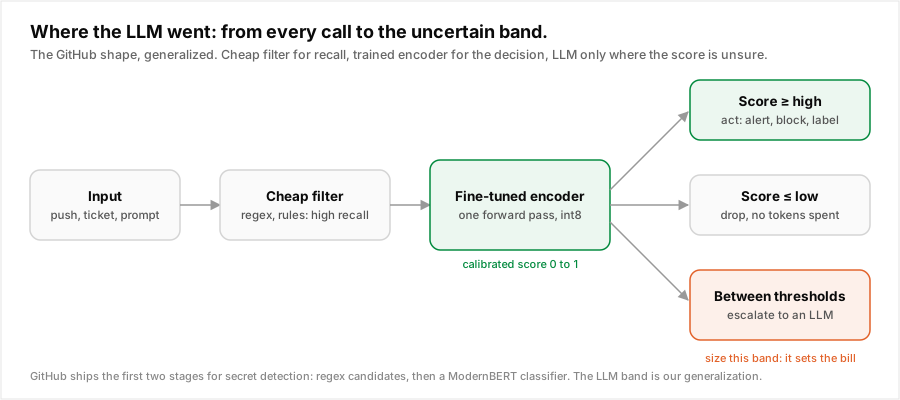
The new pipeline has two stages:
- Candidate generation. Regexes tuned for high recall flag every string that could be a credential. They're deterministic, fast and cheap, and they don't try to be precise.
- Context-aware classification. The fine-tuned ModernBERT encoder scores each candidate from the value, the file path, the secret type and a bounded window of surrounding code. Its output is a calibrated score checked against a threshold picked offline. Only high-confidence findings become alerts.
The training data came from three places: product feedback with human validation, regex candidates with human and weak labels, and synthetic hard cases (docs secrets, test fixtures, public keys, near-miss pairs) that passed deterministic and model-based checks. Before splitting into train and eval, rows were grouped by repository, candidate value and example, so near-duplicates couldn't leak from training into the test set. That one detail decides whether your offline numbers mean anything, and we come back to it in the recipe.
The rollout went offline eval on the same public traffic as the production baseline, then threshold selection, then validation on production-like traffic, then a customer A/B test against the LLM pipeline.
What the post doesn't say: which LLM it replaced, the parameter count or sequence length, dataset sizes, hardware, or absolute precision and recall. Every number is relative and measured on GitHub's own traffic. Treat the 98% as one well-run team's result, not a law. The cost math below suggests it's what you should expect.
Why the encoder wins on all three numbers.
Cost. A classification call to an LLM pays for its whole prompt every time: the instructions, the label definitions, the few-shot examples and then the item. A 1,500-token call that returns four tokens is more than 99% input. An encoder does one forward pass over a few hundred tokens of the item alone. The instructions live in its weights, and no output tokens are generated.
Speed. One forward pass on a local CPU against an API round trip plus prefill plus decoding. Running in-process also removes network jitter, rate limits and provider incidents. That's what let GitHub move detection from after the push to before it. A slower classifier would have stalled every git push.
Accuracy. This is the part people don't expect. A prompted LLM is a generalist reading a task description. A fine-tuned encoder has seen thousands of labeled examples from your distribution, including the near-misses. It also returns a probability you can calibrate, so you pick the operating point (the precision/recall trade) offline with a threshold. A prompted model gives you "yes" or "no". Asking it for a confidence number gets you a number, not a calibrated one.
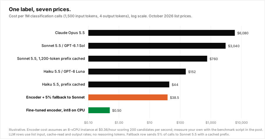
Here's what one million calls costs at October list prices, for a typical shape: a 1,200-token instruction prefix, 300 tokens of item and context, a four-token label, no reasoning.
| Classifier | Cost per 1M calls | vs encoder |
|---|---|---|
| Claude Opus 5.5 ($4 / $20) | $6,080 | 12,160x |
| Claude Sonnet 5.5 or GPT-6.1 Sol ($2 / $10) | $3,040 | 6,080x |
| Sonnet 5.5, instruction prefix cached | $760 | 1,520x |
| Claude Haiku 5.5 or GPT-6 Luna ($0.10 / $0.50) | $152 | 304x |
| Haiku 5.5, instruction prefix cached | $44 | 88x |
| Fine-tuned encoder + 5% fallback to cached Sonnet | $38.50 | 77x |
| Fine-tuned encoder, int8 on an 8-vCPU box | $0.50 | 1x |
Two things fall out of that table.
98% is the conservative end. Against the cheapest frontier-lab model with prompt caching switched on, the encoder is still 98.9% cheaper. Against a mid-tier model it's 99.98%. GitHub's ">98%" fits a baseline anywhere on the ladder.
The fallback band sets your bill, not the encoder. Send just 5% of calls back to Sonnet for the hard cases and the cost goes from $0.50 to $38.50 per million. That's still about 95% below Sonnet with caching, but it's 77 times the encoder alone. Every point of escalation rate costs more than the encoder's entire compute bill. Narrowing the uncertain band is the main cost lever after you've distilled.
Step 1: find the classifiers in your traffic.
You don't need to guess which calls are labels. They have a signature: the same system prompt, very high volume, tiny outputs, and a small set of distinct answers. This script reads a JSONL export of request logs (most gateways and observability tools can produce one) and ranks candidates by monthly spend.
# find_classifiers.py: rank classifier-shaped LLM calls by spend.
# Each log line: {"system": str, "output": str, "input_tokens": int,
#                 "output_tokens": int, "cost_usd": float}
import hashlib, json, sys
from collections import defaultdict
from statistics import median

groups = defaultdict(lambda: {"n": 0, "cost": 0.0, "out_tok": [], "answers": set(), "sample": ""})

for line in open(sys.argv[1]):
    r = json.loads(line)
    key = hashlib.sha1(r["system"].encode()).hexdigest()[:10]
    g = groups[key]
    g["n"] += 1
    g["cost"] += r["cost_usd"]
    g["out_tok"].append(r["output_tokens"])
    if len(g["answers"]) <= 50:
        g["answers"].add(r["output"].strip().lower()[:40])
    g["sample"] = g["sample"] or r["system"][:80]

days = float(sys.argv[2]) if len(sys.argv) > 2 else 30
rows = []
for key, g in groups.items():
    if g["n"] < 1000:
        continue
    shaped = median(g["out_tok"]) <= 8 and len(g["answers"]) <= 25
    if shaped:
        rows.append((g["cost"] * 30 / days, key, g["n"], len(g["answers"]), g["sample"]))

for monthly, key, n, k, sample in sorted(rows, reverse=True):
    print(f"${monthly:>10,.2f}/mo  {n:>9,} calls  {k:>2} labels  {key}  {sample!r}")
Run it on 30 days of logs. The top of the list is your shortlist. In our experience the usual suspects are routing and intent prompts ("which team owns this ticket"), moderation and policy checks, relevance filters in RAG pipelines, dedup checks, PII or secret detection, and LLM-as-judge pass/fail gates.
Don't skip the volume column. A classifier that runs 20,000 times a month isn't worth a model, as the break-even section shows.
Step 2: build the dataset, and split it honestly.
You already have labels. Every logged LLM output on a classifier-shaped prompt is a weak label. That's distillation: the LLM is the teacher, and the encoder learns to reproduce its decisions. Three upgrades turn weak labels into a dataset that can beat the teacher, which is what GitHub got:
- Fold in product feedback. Tickets re-assigned by a human, alerts dismissed as false positives, moderation decisions overturned on appeal. Those are the cases where the teacher was wrong, and they're the most valuable rows you have.
- Hand-label a disagreement sample. Run two cheap prompts or two models over a sample and hand-label wherever they disagree. A few hundred human labels on hard cases do more than ten thousand easy ones.
- Add synthetic near-misses. For every class, generate examples that look like it and aren't: the test fixture that looks like a key, the angry message that isn't an escalation. Validate them before they go in.
Then split by group, not by row. If the same customer, repository, template or document shows up in both train and eval, the model memorizes it and your offline accuracy is fiction.
from sklearn.model_selection import GroupShuffleSplit
import pandas as pd

df = pd.read_json("labeled.jsonl", lines=True)   # text, label, group (repo / customer / template id)
gss = GroupShuffleSplit(n_splits=1, test_size=0.15, random_state=7)
train_idx, test_idx = next(gss.split(df, groups=df["group"]))
df.iloc[train_idx].to_json("train.jsonl", orient="records", lines=True)
df.iloc[test_idx].to_json("test.jsonl", orient="records", lines=True)
Step 3: fine-tune ModernBERT.
ModernBERT is a 2024 encoder from Answer.AI and LightOn with an 8,192-token context. That's long enough for an item plus a real window of context, which GitHub's classifier relies on. The base model has about 150M parameters. Fine-tuning it on tens of thousands of short examples takes minutes to an hour on a single rented GPU. You need transformers 4.48 or later.
from datasets import load_dataset
from transformers import (AutoTokenizer, AutoModelForSequenceClassification,
                          TrainingArguments, Trainer)

MODEL = "answerdotai/ModernBERT-base"
ds = load_dataset("json", data_files={"train": "train.jsonl", "test": "test.jsonl"})
labels = sorted(set(ds["train"]["label"]))
l2i = {l: i for i, l in enumerate(labels)}

tok = AutoTokenizer.from_pretrained(MODEL)
def prep(b):
    enc = tok(b["text"], truncation=True, max_length=512)
    enc["labels"] = [l2i[l] for l in b["label"]]
    return enc
ds = ds.map(prep, batched=True, remove_columns=ds["train"].column_names)

model = AutoModelForSequenceClassification.from_pretrained(
    MODEL, num_labels=len(labels),
    id2label=dict(enumerate(labels)), label2id=l2i)

args = TrainingArguments("out", learning_rate=3e-5, num_train_epochs=3,
                         per_device_train_batch_size=32, bf16=True,
                         eval_strategy="epoch", save_strategy="epoch",
                         load_best_model_at_end=True)
Trainer(model=model, args=args, train_dataset=ds["train"],
        eval_dataset=ds["test"], processing_class=tok).train()
model.save_pretrained("out/best"); tok.save_pretrained("out/best")
For a binary "act or don't" task, lay out the input the way GitHub does: put the structured fields first (path: config/db.yml | type: password |) and the context window after. Fields cost a few tokens and give the model the signal a human reviewer would look at first.
Step 4: pick two thresholds, not one.
This is where the cascade comes in. Score the held-out set and choose:
- a high threshold, above which you act without asking anyone (alert, block, route, label);
- a low threshold, below which you drop the item;
- the band in between, which goes to an LLM, or to a human if the stakes call for it.
import numpy as np

def pick_band(p, y, target_precision=0.98, target_npv=0.995):
    # p: positive-class probability on held-out data, y: 0/1 truth
    hi = next(t for t in np.arange(0.50, 1.00, 0.01)
              if y[p >= t].mean() >= target_precision)
    lo = max(t for t in np.arange(0.00, 0.50, 0.01)
             if (1 - y[p <= t]).mean() >= target_npv)
    band = ((p > lo) & (p < hi)).mean()
    return round(lo, 2), round(hi, 2), band

lo, hi, band = pick_band(p_test, y_test)
print(f"drop <= {lo}, act >= {hi}, escalate {band:.1%} of traffic")
The printed band is your escalation rate, and from the cost table it's also roughly your bill. Running the encoder alone means a band of zero and a single threshold, which is what GitHub describes. Keeping a band buys a safety net while the model earns trust. Then tighten it every time you retrain on the band's LLM-labeled outputs.
Step 5: export to ONNX int8 and measure.
pip install "optimum[onnxruntime]"
optimum-cli export onnx --model out/best --task text-classification onnx/
from optimum.onnxruntime import ORTQuantizer, ORTModelForSequenceClassification
from optimum.onnxruntime.configuration import AutoQuantizationConfig
from transformers import AutoTokenizer, pipeline
import time
q = ORTQuantizer.from_pretrained("onnx/")
q.quantize(save_dir="onnx-int8/",
quantization_config=AutoQuantizationConfig.avx512_vnni(is_static=False, per_channel=False))
model = ORTModelForSequenceClassification.from_pretrained("onnx-int8/", file_name="model_quantized.onnx")
clf = pipeline("text-classification", model=model, tokenizer=AutoTokenizer.from_pretrained("out/best"))
HOURLY_PRICE = 0.36 # your instance's on-demand $/hour
texts = held_out_texts[:2000] # real items from your test split
t = time.perf_counter(); clf(texts, batch_size=32, truncation=True); dt = time.perf_counter() - t
per_s = len(texts) / dt
print(f"{per_s:,.0f} items/s -> ${HOURLY_PRICE / (per_s * 3600) * 1e6:.2f} per 1M items")Two checks before you ship:
- Re-score the test set with the int8 model and confirm precision and recall at your thresholds moved by less than a point. Dynamic quantization is usually close to lossless on encoders, but "usually" is not a release criterion.
- Put your real hourly instance price in
HOURLY_PRICE. Our chart assumes an 8-vCPU box at $0.36 an hour doing 200 items per second, which works out to $0.50 per million. Your number will differ with sequence length and hardware, but it won't move the order of magnitude.
Who should build this, and who shouldn't.
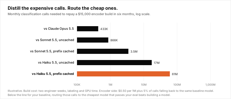
A distilled classifier has a fixed cost: labeling, a couple of engineer-weeks, GPU time, and a retraining loop as your data drifts. We put the build at $15,000 and asked how many calls a month repay it in six months, with 5% of traffic still escalating to the original model.
| Your current classifier | Saving per 1M calls | Calls per month to repay in 6 months |
|---|---|---|
| Claude Opus 5.5 | about $5,775 | 433K |
| Sonnet 5.5, uncached | about $2,887 | 866K |
| Sonnet 5.5, prefix cached | about $722 | 3.5M |
| Haiku 5.5, uncached | about $144 | 17M |
| Haiku 5.5, prefix cached | about $41 | 61M |
Read the table from both ends.
- If a frontier or mid-tier model is classifying at volume, build the encoder. Under a million calls a month to repay it, plus the latency win, plus a likely accuracy win. This is GitHub's case.
- If you're under the line, route instead of building. A team doing 2M classifications a month on uncached Sonnet gets most of the saving by moving that prompt to Haiku 5.5 or GPT-6 Luna with the prefix cached: $3,040 down to $44 per million, with no model to own. The encoder would add another $41 per million at that point, about $80 a month on 2M calls. Not worth a training pipeline.
- If the "label" needs reasoning, don't distill it. Judging whether a long agent transcript achieved its goal, or whether a contract clause conflicts with a policy, isn't a pattern over a few hundred tokens. Keep an LLM, and route it by difficulty.
- If the label set changes weekly, wait. An encoder bakes the labels into its head. Brand-new categories every sprint means retraining every sprint. Zero-shot models handle that better, at a cost. We benchmarked that trade in Where the Label Lives.
The general lesson.
GitHub didn't make its LLM cheaper. It noticed that one stage of its pipeline wasn't asking a generative question, and gave that stage a model shaped like the answer. The 98% came from changing the shape, not from negotiating a price.
Most teams that audit their LLM spend find the same split. A small set of calls really needs a frontier model. A big set needs a cheaper model. And a surprising slice doesn't need generation at all: it's decisions that happen to be phrased as prompts. Fine-tuning versus routing for the middle tier is covered in Fine-Tune or Route. The same logic applies here one level down.
Where Nadir fits.
Nadir is built on exactly this split, and we use it on ourselves. The decision of which model should answer a prompt is a classification, so it doesn't go to an LLM. POST /v1/bucket returns simple, medium or complex with a probability for each, from a trained classifier, without spending provider tokens. We wrote up why it's a trained head and not a prompted model in How our binary classifier routes prompts in 50ms.
For everything that stays generative, Nadir's OpenAI compatible gateway does the routing half of the table above. Send model="auto" and each prompt goes to the cheapest model you've configured that clears the quality floor you set per API key. Every response reports which model answered and what it cost. That per-call log is also the input to Step 1: a week of traffic through Nadir shows you which prompts are classifier-shaped, how often they run and what they cost, so you know which ones to distill and which ones routing already handles.
Start with a free key, point a week of traffic at it in Observe mode (it records the decision Nadir would make without changing a single response), and sort your spend by prompt. The decisions dressed up as generation are usually near the top.
Sources: GitHub Blog, ["GitHub's model for secret detection: Finding more secrets with less noise"](https://github.blog/ai-and-ml/githubs-model-for-secret-detection-finding-more-secrets-with-less-noise/), Batu Ozturkler and Shengyu Fu, October 13, 2026, for the pipeline design, training data, rollout and every GitHub figure (98%, 86%, 13%, 19%, 11.5%). [Help Net Security coverage](https://www.helpnetsecurity.com/?p=387865) of the same announcement. ModernBERT: Warner et al., ["Smarter, Better, Faster, Longer"](https://arxiv.org/abs/2412.13663), December 2024. Model prices from our [October 2026 LLM API pricing comparison](/blog/llm-api-pricing-june-2026-complete-comparison). The call shape, encoder throughput and instance price, the 5% fallback, the $15,000 build cost, every cost-per-million and break-even figure, and all three charts are our own illustrative calculations.