TL;DR.
On October 7, 2026, Weave published a new series in its index: return on token spend, the engineering output a dollar of AI tool spend buys. In January 2026 a dollar bought 0.352 estimated expert hours of merged code. In September it bought 0.106. That's a 70% drop in eight months. Put the other way round, the AI spend behind one expert hour of output went from $2.84 to $9.39.
Two days later, G2 published interviews with US enterprise LLM buyers. 53% have no formal metric for what a unit of AI work costs. Only 15% said cost drove their latest model change.
Put those together and you get the 2026 AI budget in one sentence: spend is growing faster than what it buys, and most companies can't see it, because they track the bill and not the ratio.
This post covers:
- What the Weave number measures, and what it doesn't
- Why a falling average return means the marginal dollar is worth much less
- The three explanations for the slide, and how to tell which one is yours
- A Python tutorial: compute your own return on token spend, your spend elasticity, and how much of the denominator is paying frontier prices for work a cheaper model handles
Weave's figures are aggregate customer telemetry, not a controlled study, and the output unit is modeled. G2's are AI-led interviews with small bases. Treat both as direction. The tutorial runs on synthetic data, not Nadir customer data.
The number.
Weave measures engineering output in one unit: the time an expert engineer would need to complete each merged pull request. It divides total output by total attributed AI tool spend, counting only engineers who had both in the same month. Spend that can't be pinned to a person, like org-level overage charges, is left out.
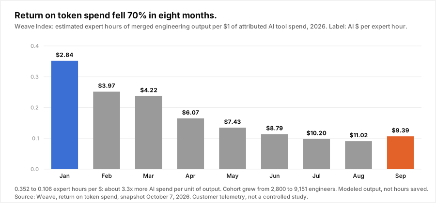
| Month (2026) | Expert hours per $ | AI $ per expert hour |
|---|---|---|
| January | 0.352 | $2.84 |
| March | 0.237 | $4.22 |
| May | 0.135 | $7.43 |
| July | 0.098 | $10.20 |
| August | 0.091 | $11.02 |
| September | 0.106 | $9.39 |
Three things to read off it before reading anything into it.
$9.39 per expert hour is still cheap. A loaded senior engineer costs well over $100 an hour. AI tools didn't stop paying for themselves this year, and this post isn't arguing they did. The slide is about the trend and where it's heading, not about whether to use AI at all.
The fall is steady, not a one-off. Seven months of decline in a row, with a small rebound in September. That's not a pricing event, like one model getting more expensive. Something structural changed in how the spend was used.
The cohort tripled. 2,800 engineers in January, 9,151 in September. Weave says itself that changes in the cohort and connected telemetry can move the series, and that the data alone doesn't show AI caused any change in output. January's cohort was early adopters with broad telemetry. September's includes everyone who joined since.
The average hides the last dollar.
A 70% fall in the average is the gentle version. What a budget owner actually decides is the next dollar, and when returns are diminishing, the next dollar is always worth less than the average.
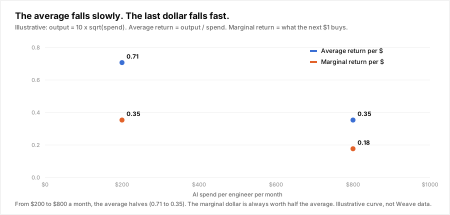
With an illustrative curve where output grows with the square root of spend, an engineer going from $200 to $800 a month halves the average return. The marginal return, what the last dollar bought, was half the average the whole way down. At $800 a month, the last dollar buys a quarter of what the first $200 bought on average.
That's what "tokenmaxxing" looks like in a chart. We wrote about the behavior in tokenmaxxing and about the macro version in the AI Jevons paradox: when tokens are cheap and usage is rewarded, spend grows into the work at the low-value end first.
You can measure your own curve. The tutorial below fits it from one month of per-engineer data.
Three reasons it falls.
A ratio falls when the denominator grows faster than the numerator. In AI spend, three different stories produce the same chart, and they need different fixes.
| Explanation | What you'd see in your own data | Fix |
|---|---|---|
| Diminishing returns. More agent runs, more retries, more parallel attempts, each adding less | Output per engineer flat or slow, requests and tokens per engineer climbing | Caps on loops and retries, cost per resolved task as the target |
| Price mix. The same work moved to pricier models, longer contexts, reasoning effort and fast tiers | Tokens per task roughly flat, $ per token climbing | Route each request to the cheapest model that can handle it |
| Composition. New, later adopters and new kinds of work entering the cohort | Return falls in aggregate, holds per engineer over time | Compare matched cohorts before acting |
Most teams have all three. The point is that the fix for one is waste for another. A spend cap is the right tool for runaway loops and the wrong tool for price mix: it cuts the useful work along with the overpriced work. We covered why caps misfire in spend caps are not cost cuts.
The price-mix story deserves the most suspicion in 2026, because the defaults moved up all year. Agentic coding tools default to flagship models. Reasoning effort defaults went up. Context windows got longer and past pricing cliffs. Fast tiers arrived at 6x the price. None of that requires anyone to do more work. It just reprices the same work.
What the buyers measure instead.
The G2 interviews explain why the slide went unnoticed in so many companies:
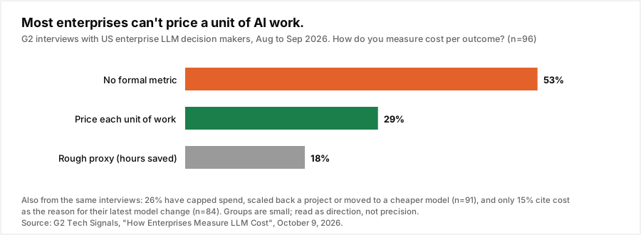
| G2 finding (US enterprise LLM buyers) | Share | Base |
|---|---|---|
| Compare models on ROI and labor savings | 60% | 98 |
| Compare on total spend and token efficiency | 23% | 98 |
| No formal cost-per-outcome metric | 53% | 96 |
| Capped spend, scaled back, or moved to a cheaper model | 26% | 91 |
| Latest model change driven by cost | 15% | 84 |
| Latest model change driven by performance | 57% | 84 |
Of 102 leaders, 68 used the word "token" and one reasoned from the price per million tokens. The leaders who did have a unit cost had good ones: one SaaS team runs AI support at about $1 per ticket against $50 or more for a human interaction.
That's the gap. The ratio Weave tracks at the market level is the ratio each company should track for itself, and half don't. A bill that grows 3x while output grows 1x looks the same on an invoice as a bill that grows 3x while output grows 3x.
On October 9, Oracle India's Vivek Gupta put the same idea into a formula: divide total monthly AI spend, including retrieval, storage, monitoring and human review, by completed workflow outcomes. It's a recommendation rather than a benchmark, but it's the right denominator flip.
Tutorial: measure your own return on token spend.
You need two tables for a month:
- Spend per person (or team, or service) from your gateway or provider billing, attributed by key or header
- Output per person in whatever unit your org already trusts: merged PRs weighted by size, resolved tickets, completed workflows, documents reviewed
If you haven't attributed spend yet, start with who spent the tokens. The rest is about 60 lines of Python, standard library only.
Step 1: the ratio, both ways.
import math
from collections import defaultdict

def return_on_spend(rows):
    """rows: dicts with engineer, spend_usd, output_units for one month."""
    spend = sum(r["spend_usd"] for r in rows)
    output = sum(r["output_units"] for r in rows)
    return output / spend, spend / output   # units per $, $ per unit
Report both. "Units per dollar" is the return. "Dollars per unit" is what finance will ask for, and it's the one that matches a $1-per-ticket style number.
Step 2: is the next dollar worth it?
Fit output against spend across engineers on a log-log scale. The slope b is your spend elasticity: how much output rises, in percent, when spend rises 1%.
def spend_elasticity(rows):
    """Fit output = a * spend^b across engineers. b < 1 means diminishing
    returns, and marginal return = b * average return."""
    pts = [(math.log(r["spend_usd"]), math.log(r["output_units"]))
           for r in rows if r["spend_usd"] > 0 and r["output_units"] > 0]
    n = len(pts)
    mx = sum(x for x, _ in pts) / n
    my = sum(y for _, y in pts) / n
    return (sum((x - mx) * (y - my) for x, y in pts)
            / sum((x - mx) ** 2 for x, _ in pts))

def by_band(rows, bands=4):
    rows = sorted(rows, key=lambda r: r["spend_usd"])
    size = math.ceil(len(rows) / bands)
    out = []
    for i in range(0, len(rows), size):
        chunk = rows[i:i + size]
        units_per_usd, _ = return_on_spend(chunk)
        out.append((chunk[0]["spend_usd"], chunk[-1]["spend_usd"], units_per_usd))
    return out
b near 1 means spend scales with output: every dollar buys about what the average dollar buys. b near 0.5 means the marginal dollar buys half the average. The spend bands show the same thing without a model: if your top quartile of spenders gets a third of the return of your bottom quartile, that's the curve.
One caution: this is a cross-section, not an experiment. High spenders may simply do different work, like large migrations where AI is less useful per dollar. Use it to find where to look, not to set a cap per person.
Step 3: how much of the denominator is price mix?
This is the part a cap can't fix and routing can. Take a sample of requests, label each with the cheapest tier that handles that kind of request, and reprice. The label can come from your own evals, or from a classifier such as Nadir's /v1/bucket, which returns simple, medium or complex with a probability for each.
# $ per 1M tokens (input, output). List prices as of October 12, 2026,
# prompts under each model's long-context threshold. Use your own rate card.
PRICE = {
    "haiku-5.5":  (0.10, 0.50),
    "sonnet-5.5": (2.00, 10.00),
    "opus-5.5":   (4.00, 20.00),
}
ORDER = ["haiku-5.5", "sonnet-5.5", "opus-5.5"]

def cost(model, tokens_in, tokens_out):
    pin, pout = PRICE[model]
    return (tokens_in * pin + tokens_out * pout) / 1e6

def routing_headroom(requests):
    """requests: dicts with served, needed, tokens_in, tokens_out."""
    actual = repriced = 0.0
    over = defaultdict(float)
    for r in requests:
        c = cost(r["served"], r["tokens_in"], r["tokens_out"])
        tier = min(r["served"], r["needed"], key=ORDER.index)
        c2 = cost(tier, r["tokens_in"], r["tokens_out"])
        actual += c
        repriced += c2
        if tier != r["served"]:
            over[(r["served"], tier)] += c - c2
    return actual, repriced, dict(over)
The min matters: never reprice a request up. If something was served on a cheap model and needed a bigger one, that's a quality problem to look at separately, not a saving.
Step 4: read it together.
units_per_usd, usd_per_unit = return_on_spend(month_rows)
b = spend_elasticity(month_rows)
actual, repriced, over = routing_headroom(request_sample)

print(f"return: {units_per_usd:.3f} units/$ (${usd_per_unit:.2f} per unit)")
print(f"elasticity: {b:.2f}, marginal return {b * units_per_usd:.3f} units/$")
for lo, hi, r in by_band(month_rows):
    print(f"  ${lo:,.0f} to ${hi:,.0f} per month: {r:.3f} units/$")
print(f"price-mix headroom: {1 - repriced / actual:.0%} of sampled spend")
On a synthetic month of 200 engineers with output growing as spend to the power 0.45, it prints:
return: 0.233 units/$ ($4.29 per unit)
elasticity: 0.47, marginal return 0.110 units/$
  $60 to $314 per month: 0.489 units/$
  $317 to $671 per month: 0.289 units/$
  $685 to $1,051 per month: 0.224 units/$
  $1,061 to $1,485 per month: 0.180 units/$
The fit recovers the 0.45 we put in, and the top band returns about a third of the bottom one. The headroom line depends entirely on your traffic mix, so we're not printing a synthetic one. Run it on a real sample. If it's small, your slide is diminishing returns or composition, and caps on loops and retries are the lever. If it's large, a lot of your denominator is paying flagship prices for work that didn't need them.
What to put on the monthly report.
| Metric | Why |
|---|---|
| $ per unit of output, per team | The number finance actually wants, and the one that catches a 3x bill on 1x output |
Spend elasticity b | Below about 0.5, new budget mostly buys low-value usage |
| Price-mix headroom | Spend you can remove without removing any work |
| Share of spend on flagship models and fast tiers | The leading indicator for price mix, before it shows up in the ratio |
Where Nadir fits.
There are two ways to lift return on token spend: more output per dollar, or fewer dollars per output. The first is a workflow problem, and it's slow. The second is mostly a routing problem, and it's a config change.
Nadir works on the denominator. Send model="auto" and a trained classifier reads each prompt and sends it to the cheapest model that can handle it, among the models you've configured and against the quality floor you set on the API key. The work and the output stay the same. Each response reports the model served and its cost, attributed by key and by the X-Nadir-Use-Case and X-Nadir-Tags headers, so Step 1 of the tutorial is a dashboard view rather than a data project. How much it saves depends on your mix, which is exactly what Step 3 measures.
If you'd rather not change any traffic yet, Observe mode records the routing decision Nadir would make on every request without altering a response. That's the needed column in Step 3, filled in on your real traffic. Start with a free key.
Routing doesn't fix everything on this list. It won't stop an agent loop that runs forty turns when four would do, and it won't fix a cohort that adopted tools without a use for them. For the loops, see the stopping problem. For the price mix, routing is the direct fix.
Conclusion.
Weave's index says the market's AI dollar bought 70% less engineering output in September than in January. That's still a good deal at $9.39 an expert hour, but the trend matters more than the level, and the marginal dollar is worth less than the average one. Half of enterprise buyers can't see any of this, because they track the bill instead of the ratio. Track the ratio. Fit the curve. Then split the slide into its three causes, because the fix for price mix is routing, the fix for runaway loops is a stopping rule, and the fix for neither is a blanket cap.
Sources: Weave, ["Return on token spend"](https://weaveos.com/data/return-on-token-spend), Weave Index snapshot updated October 7, 2026, aggregate customer telemetry, January to September 2026; Emilie Audubert, ["How Enterprises Measure LLM Cost: 53% Still Have No Formal Metric"](https://learn.g2.com/tech-signals-cost-per-outcome-llms), G2 Tech Signals, October 9, 2026, 102 AI-led interviews with US enterprise leaders, August and September 2026; Express Computer, ["Start with the outcome: Oracle India's Vivek Gupta on taking AI from pilot to production"](https://www.expresscomputer.in/news/start-with-the-outcome-oracle-indias-vivek-gupta-on-taking-ai-from-pilot-to-production/139678/), October 9, 2026. Found via [Token Cost Radar](https://jcodemunch.com/radar/2026-10-10), October 10, 2026. The average-versus-marginal curve and the tutorial data are illustrative and are not Weave's, G2's or Nadir customers' figures. Model prices are list prices as of October 12, 2026.